Chemmy's Blog

Thu Aug 08 2019 00:00:00 GMT+0800 (China Standard Time)

发表于 2019-08-08 更新于 2026-03-05

wpa_supplicant及wpa_cli使用方法

发表于 2019-08-04 更新于 2026-03-05 分类于 Linux

wpa_supplicant是一个连接、配置WIFI的工具，它主要包含wpa_supplicant与wpa_cli两个程序。通常情况下，可以通过wpa_cli来进行WIFI的配置与连接，如果有特殊的需要，可以编写应用程序直接调用wpa_supplicant的接口直接开发。

启动`wpa_supplicant`应用

1	$ wpa_supplicant -D nl80211 -i wlan0 -c /etc/wpa_supplicant.conf -B

/etc/wpa_supplicant.conf文件里，添加下面代码:

1	ctrl_interface=/var/run/wpa_supplicant update_config=1

启动`wpa_cli`应用

1
2
3

$ wpa_cli -i wlan0 scan # 搜索附近wifi网络 
$ wpa_cli -i wlan0 scan_result # 打印搜索wifi网络结果 
$ wpa_cli -i wlan0 add_network # 添加一个网络连接

如果要连接加密方式是[WPA-PSK-CCMP+TKIP][WPA2-PSK-CCMP+TKIP][ESS] (wpa加密)，wifi名称是name，wifi密码是：psk。

1
2
3

$ wpa_cli -i wlan0 set_network 0 ssid '"name"' 
$ wpa_cli -i wlan0 set_network 0 psk '"psk"' 
$ wpa_cli -i wlan0 enable_network 0

如果要连接加密方式是[WEP][ESS] (wep加密)，wifi名称是name，wifi密码是psk。

$ wpa_cli -i wlan0 set_network 0 ssid '"name"' 
$ wpa_cli -i wlan0 set_network 0 key_mgmt NONE 
$ wpa_cli -i wlan0 set_network 0 wep_key0 '"psk"' 
$ wpa_cli -i wlan0 enable_network 0

如果要连接加密方式是[ESS] (无加密)，wifi名称是name。

1
2
3

$ wpa_cli -i wlan0 set_network 0 ssid '"name"' 
$ wpa_cli -i wlan0 set_network 0 key_mgmt NONE 
$ wpa_cli -i wlan0 enable_network 0

分配`ip/netmask/gateway/dns`

1	$ udhcpc -i wlan0 -s /etc/udhcpc.script -q

执行完毕，就可以连接网络了。

保存连接

1	$ wpa_cli -i wlan0 save_config

断开连接

1	$ wpa_cli -i wlan0 disable_network 0

连接已有的连接

1
2
3

$ wpa_cli -i wlan0 list_network #列举所有保存的连接 
$ wpa_cli -i wlan0 select_network 0 #连接第1个保存的连接 
$ wpa_cli -i wlan0 enable_network 0 #使能第1个保存的连接

断开`wifi`

1
2
3

$ ifconfig wlan0 down 
$ killall udhcpc 
$ killall wpa_supplicant

`wpa_wifi_tool`使用方法

wpa_wifi_tool是基于wpa_supplicant及wpa_cli的一个用于快速设置wifi的工具，方便调试时连接wifi使用。使用方法：1、运行wpa_wifi_tool;2、输入help进行命令查看;3、s进行SSID扫描;4、c[n]进行wifi连接，连接时若为新的SSID则需输入密码，若为已保存的SSID则可以使用保存过的密码或者重新输入密码;5、e退出工具。

Sat Aug 03 2019 00:00:00 GMT+0800 (China Standard Time)

发表于 2019-08-03 更新于 2026-03-05

Windows InfluxDB 安装与配置

发表于 2019-08-03 更新于 2026-03-05 分类于数据库， InfluxDB

一、下载链接https://portal.influxdata.com/downloads，选windows版

二、解压到安装盘，目录如下

三、修改conf文件，代码如下，直接复制粘贴（1.4.2版本），注意修改路径，带D盘的改为你的安装路径就好，一共三个，注意网上有配置admin进行web管理，但新版本配置文件里没有admin因为官方给删除了，需下载Chronograf，后文会介绍

### Welcome to the InfluxDB configuration file.

# The values in this file override the default values used by the system if
# a config option is not specified. The commented out lines are the configuration
# field and the default value used. Uncommenting a line and changing the value
# will change the value used at runtime when the process is restarted.

# Once every 24 hours InfluxDB will report usage data to usage.influxdata.com
# The data includes a random ID, os, arch, version, the number of series and other
# usage data. No data from user databases is ever transmitted.
# Change this option to true to disable reporting.
# reporting-disabled = false

# Bind address to use for the RPC service for backup and restore.
# bind-address = "127.0.0.1:8088"

###
### [meta]
###
### Controls the parameters for the Raft consensus group that stores metadata
### about the InfluxDB cluster.
###

[meta]
  # Where the metadata/raft database is stored
  dir = "D:/influxdb-1.4.2-1/meta"

  # Automatically create a default retention policy when creating a database.
    retention-autocreate = true

  # If log messages are printed for the meta service
    logging-enabled = true

###
### [data]
###
### Controls where the actual shard data for InfluxDB lives and how it is
### flushed from the WAL. "dir" may need to be changed to a suitable place
### for your system, but the WAL settings are an advanced configuration. The
### defaults should work for most systems.
###

[data]
  # The directory where the TSM storage engine stores TSM files.
  dir = "D:/influxdb-1.4.2-1/data"

  # The directory where the TSM storage engine stores WAL files.
  wal-dir = "D:/influxdb-1.4.2-1/wal"

  # The amount of time that a write will wait before fsyncing.  A duration
  # greater than 0 can be used to batch up multiple fsync calls.  This is useful for slower
  # disks or when WAL write contention is seen.  A value of 0s fsyncs every write to the WAL.
  # Values in the range of 0-100ms are recommended for non-SSD disks.
  # wal-fsync-delay = "0s"


  # The type of shard index to use for new shards.  The default is an in-memory index that is
  # recreated at startup.  A value of "tsi1" will use a disk based index that supports higher
  # cardinality datasets.
  # index-version = "inmem"

  # Trace logging provides more verbose output around the tsm engine. Turning
  # this on can provide more useful output for debugging tsm engine issues.
  # trace-logging-enabled = false

  # Whether queries should be logged before execution. Very useful for troubleshooting, but will
  # log any sensitive data contained within a query.
    query-log-enabled = true

  # Settings for the TSM engine

  # CacheMaxMemorySize is the maximum size a shard's cache can
  # reach before it starts rejecting writes.
  # Valid size suffixes are k, m, or g (case insensitive, 1024 = 1k).
  # Vaues without a size suffix are in bytes.
  # cache-max-memory-size = "1g"

  # CacheSnapshotMemorySize is the size at which the engine will
  # snapshot the cache and write it to a TSM file, freeing up memory
  # Valid size suffixes are k, m, or g (case insensitive, 1024 = 1k).
  # Values without a size suffix are in bytes.
  # cache-snapshot-memory-size = "25m"

  # CacheSnapshotWriteColdDuration is the length of time at
  # which the engine will snapshot the cache and write it to
  # a new TSM file if the shard hasn't received writes or deletes
  # cache-snapshot-write-cold-duration = "10m"

  # CompactFullWriteColdDuration is the duration at which the engine
  # will compact all TSM files in a shard if it hasn't received a
  # write or delete
  # compact-full-write-cold-duration = "4h"

  # The maximum number of concurrent full and level compactions that can run at one time.  A
  # value of 0 results in 50% of runtime.GOMAXPROCS(0) used at runtime.  Any number greater
  # than 0 limits compactions to that value.  This setting does not apply
  # to cache snapshotting.
  # max-concurrent-compactions = 0

  # The maximum series allowed per database before writes are dropped.  This limit can prevent
  # high cardinality issues at the database level.  This limit can be disabled by setting it to
  # 0.
  # max-series-per-database = 1000000

  # The maximum number of tag values per tag that are allowed before writes are dropped.  This limit
  # can prevent high cardinality tag values from being written to a measurement.  This limit can be
  # disabled by setting it to 0.
  # max-values-per-tag = 100000

###
### [coordinator]
###
### Controls the clustering service configuration.
###

[coordinator]
  # The default time a write request will wait until a "timeout" error is returned to the caller.
  # write-timeout = "10s"

  # The maximum number of concurrent queries allowed to be executing at one time.  If a query is
  # executed and exceeds this limit, an error is returned to the caller.  This limit can be disabled
  # by setting it to 0.
  # max-concurrent-queries = 0

  # The maximum time a query will is allowed to execute before being killed by the system.  This limit
  # can help prevent run away queries.  Setting the value to 0 disables the limit.
  # query-timeout = "0s"

  # The time threshold when a query will be logged as a slow query.  This limit can be set to help
  # discover slow or resource intensive queries.  Setting the value to 0 disables the slow query logging.
  # log-queries-after = "0s"

  # The maximum number of points a SELECT can process.  A value of 0 will make
  # the maximum point count unlimited.  This will only be checked every second so queries will not
  # be aborted immediately when hitting the limit.
  # max-select-point = 0

  # The maximum number of series a SELECT can run.  A value of 0 will make the maximum series
  # count unlimited.
  # max-select-series = 0

  # The maxium number of group by time bucket a SELECT can create.  A value of zero will max the maximum
  # number of buckets unlimited.
  # max-select-buckets = 0

###
### [retention]
###
### Controls the enforcement of retention policies for evicting old data.
###

[retention]
  # Determines whether retention policy enforcement enabled.
    enabled = true

  # The interval of time when retention policy enforcement checks run.
    check-interval = "30m"

###
### [shard-precreation]
###
### Controls the precreation of shards, so they are available before data arrives.
### Only shards that, after creation, will have both a start- and end-time in the
### future, will ever be created. Shards are never precreated that would be wholly
### or partially in the past.

[shard-precreation]
  # Determines whether shard pre-creation service is enabled.
    enabled = true

  # The interval of time when the check to pre-create new shards runs.
    check-interval = "10m"

  # The default period ahead of the endtime of a shard group that its successor
  # group is created.
    advance-period = "30m"

###
### Controls the system self-monitoring, statistics and diagnostics.
###
### The internal database for monitoring data is created automatically if
### if it does not already exist. The target retention within this database
### is called 'monitor' and is also created with a retention period of 7 days
### and a replication factor of 1, if it does not exist. In all cases the
### this retention policy is configured as the default for the database.

[monitor]
  # Whether to record statistics internally.
    store-enabled = true

  # The destination database for recorded statistics
    store-database = "_internal"

  # The interval at which to record statistics
    store-interval = "10s"

###
### [http]
###
### Controls how the HTTP endpoints are configured. These are the primary
### mechanism for getting data into and out of InfluxDB.
###

[http]
  # Determines whether HTTP endpoint is enabled.
    enabled = true

  # The bind address used by the HTTP service.
    bind-address = ":8086"

  # Determines whether user authentication is enabled over HTTP/HTTPS.
  # auth-enabled = false

  # The default realm sent back when issuing a basic auth challenge.
  # realm = "InfluxDB"

  # Determines whether HTTP request logging is enabled.
  # log-enabled = true

  # Determines whether detailed write logging is enabled.
  # write-tracing = false

  # Determines whether the pprof endpoint is enabled.  This endpoint is used for
  # troubleshooting and monitoring.
  # pprof-enabled = true

  # Determines whether HTTPS is enabled.
  # https-enabled = false

  # The SSL certificate to use when HTTPS is enabled.
  # https-certificate = "/etc/ssl/influxdb.pem"

  # Use a separate private key location.
  # https-private-key = ""

  # The JWT auth shared secret to validate requests using JSON web tokens.
  # shared-secret = ""

  # The default chunk size for result sets that should be chunked.
  # max-row-limit = 0

  # The maximum number of HTTP connections that may be open at once.  New connections that
  # would exceed this limit are dropped.  Setting this value to 0 disables the limit.
  # max-connection-limit = 0

  # Enable http service over unix domain socket
  # unix-socket-enabled = false

  # The path of the unix domain socket.
  # bind-socket = "/var/run/influxdb.sock"

  # The maximum size of a client request body, in bytes. Setting this value to 0 disables the limit.
  # max-body-size = 25000000


###
### [ifql]
###
### Configures the ifql RPC API.
###

[ifql]
  # Determines whether the RPC service is enabled.
  # enabled = true

  # Determines whether additional logging is enabled.
  # log-enabled = true

  # The bind address used by the ifql RPC service.
  # bind-address = ":8082"


###
### [subscriber]
###
### Controls the subscriptions, which can be used to fork a copy of all data
### received by the InfluxDB host.
###

[subscriber]
  # Determines whether the subscriber service is enabled.
  # enabled = true

  # The default timeout for HTTP writes to subscribers.
  # http-timeout = "30s"

  # Allows insecure HTTPS connections to subscribers.  This is useful when testing with self-
  # signed certificates.
  # insecure-skip-verify = false

  # The path to the PEM encoded CA certs file. If the empty string, the default system certs will be used
  # ca-certs = ""

  # The number of writer goroutines processing the write channel.
  # write-concurrency = 40

  # The number of in-flight writes buffered in the write channel.
  # write-buffer-size = 1000


###
### [[graphite]]
###
### Controls one or many listeners for Graphite data.
###

[[graphite]]
  # Determines whether the graphite endpoint is enabled.
  # enabled = false
  # database = "graphite"
  # retention-policy = ""
  # bind-address = ":2003"
  # protocol = "tcp"
  # consistency-level = "one"

  # These next lines control how batching works. You should have this enabled
  # otherwise you could get dropped metrics or poor performance. Batching
  # will buffer points in memory if you have many coming in.

  # Flush if this many points get buffered
  # batch-size = 5000

  # number of batches that may be pending in memory
  # batch-pending = 10

  # Flush at least this often even if we haven't hit buffer limit
  # batch-timeout = "1s"

  # UDP Read buffer size, 0 means OS default. UDP listener will fail if set above OS max.
  # udp-read-buffer = 0

  ### This string joins multiple matching 'measurement' values providing more control over the final measurement name.
  # separator = "."

  ### Default tags that will be added to all metrics.  These can be overridden at the template level
  ### or by tags extracted from metric
  # tags = ["region=us-east", "zone=1c"]

  ### Each template line requires a template pattern.  It can have an optional
  ### filter before the template and separated by spaces.  It can also have optional extra
  ### tags following the template.  Multiple tags should be separated by commas and no spaces
  ### similar to the line protocol format.  There can be only one default template.
  # templates = [
  #   "*.app env.service.resource.measurement",
  #   # Default template
  #   "server.*",
  # ]

###
### [collectd]
###
### Controls one or many listeners for collectd data.
###

[[collectd]]
  # enabled = false
  # bind-address = ":25826"
  # database = "collectd"
  # retention-policy = ""
  #
  # The collectd service supports either scanning a directory for multiple types
  # db files, or specifying a single db file.
  # typesdb = "/usr/local/share/collectd"
  #
  # security-level = "none"
  # auth-file = "/etc/collectd/auth_file"

  # These next lines control how batching works. You should have this enabled
  # otherwise you could get dropped metrics or poor performance. Batching
  # will buffer points in memory if you have many coming in.

  # Flush if this many points get buffered
  # batch-size = 5000

  # Number of batches that may be pending in memory
  # batch-pending = 10

  # Flush at least this often even if we haven't hit buffer limit
  # batch-timeout = "10s"

  # UDP Read buffer size, 0 means OS default. UDP listener will fail if set above OS max.
  # read-buffer = 0

  # Multi-value plugins can be handled two ways.
  # "split" will parse and store the multi-value plugin data into separate measurements
  # "join" will parse and store the multi-value plugin as a single multi-value measurement.
  # "split" is the default behavior for backward compatability with previous versions of influxdb.
  # parse-multivalue-plugin = "split"
###
### [opentsdb]
###
### Controls one or many listeners for OpenTSDB data.
###

[[opentsdb]]
  # enabled = false
  # bind-address = ":4242"
  # database = "opentsdb"
  # retention-policy = ""
  # consistency-level = "one"
  # tls-enabled = false
  # certificate= "/etc/ssl/influxdb.pem"

  # Log an error for every malformed point.
  # log-point-errors = true

  # These next lines control how batching works. You should have this enabled
  # otherwise you could get dropped metrics or poor performance. Only points
  # metrics received over the telnet protocol undergo batching.

  # Flush if this many points get buffered
  # batch-size = 1000

  # Number of batches that may be pending in memory
  # batch-pending = 5

  # Flush at least this often even if we haven't hit buffer limit
  # batch-timeout = "1s"

###
### [[udp]]
###
### Controls the listeners for InfluxDB line protocol data via UDP.
###

[[udp]]
  # enabled = false
  # bind-address = ":8089"
  # database = "udp"
  # retention-policy = ""

  # These next lines control how batching works. You should have this enabled
  # otherwise you could get dropped metrics or poor performance. Batching
  # will buffer points in memory if you have many coming in.

  # Flush if this many points get buffered
  # batch-size = 5000

  # Number of batches that may be pending in memory
  # batch-pending = 10

  # Will flush at least this often even if we haven't hit buffer limit
  # batch-timeout = "1s"

  # UDP Read buffer size, 0 means OS default. UDP listener will fail if set above OS max.
  # read-buffer = 0

###
### [continuous_queries]
###
### Controls how continuous queries are run within InfluxDB.
###

[continuous_queries]
  # Determines whether the continuous query service is enabled.
  # enabled = true

  # Controls whether queries are logged when executed by the CQ service.
  # log-enabled = true

  # Controls whether queries are logged to the self-monitoring data store.
  # query-stats-enabled = false

  # interval for how often continuous queries will be checked if they need to run
  # run-interval = "1s"

四、使配置生效并打开数据库连接，双击influxd.exe就好，然后双击influx.exe进行操作，网上有操作教程，注意操作数据库时不能关闭influxd.exe，我不知道为什么总有这么个提示：There was an error writing history file: open : The system cannot find the file specified.不过好像没啥影响

五、要使用web管理需要下载Chronograf，https://portal.influxdata.com/downloads第三个就是，下载完直接解压，双击exe程序，在浏览器输入http://localhost:8888/，一开始登录要账户密码，我都用admin就进去了

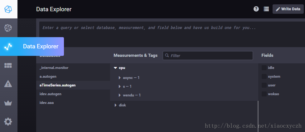
这个是查看建立的数据库

这个是查看数据库的数据

没了

Mon Jul 29 2019 00:00:00 GMT+0800 (China Standard Time)

发表于 2019-07-29 更新于 2026-03-05

git subtree教程

发表于 2019-07-27 更新于 2026-03-05 分类于 Git

关于子仓库或者说是仓库共用，git官方推荐的工具是git subtree。我自己也用了一段时间的git subtree，感觉比git submodule好用，但是也有一些缺点，在可接受的范围内。
所以对于仓库共用，在git subtree 与 git submodule之中选择的话，我推荐git subtree。

git subtree 可以实现一个仓库作为其他仓库的子仓库。

使用git subtree 有以下几个原因：

旧版本的git也支持(最老版本可以到 v1.5.2).
git subtree与git submodule不同，它不增加任何像.gitmodule这样的新的元数据文件.
git subtree对于项目中的其他成员透明，意味着可以不知道git subtree的存在.

当然，git subtree也有它的缺点，但是这些缺点还在可以接受的范围内：

必须学习新的指令(如：git subtree).
子仓库的更新与推送指令相对复杂。

git subtree的主要命令有：

git subtree add   --prefix=<prefix> <commit>
git subtree add   --prefix=<prefix> <repository> <ref>
git subtree pull  --prefix=<prefix> <repository> <ref>
git subtree push  --prefix=<prefix> <repository> <ref>
git subtree merge --prefix=<prefix> <commit>
git subtree split --prefix=<prefix> [OPTIONS] [<commit>]

准备

我们先准备一个仓库叫photoshop，一个仓库叫libpng，然后我们希望把libpng作为photoshop的子仓库。
photoshop的路径为https://github.com/test/photoshop.git，仓库里的文件有：

photoshop
    |
    |-- photoshop.c
    |-- photoshop.h
    |-- main.c
    \-- README.md

libPNG的路径为https://github.com/test/libpng.git，仓库里的文件有：

libpng
    |
    |-- libpng.c
    |-- libpng.h
    \-- README.md

以下操作均位于父仓库的根目录中。

在父仓库中新增子仓库

我们执行以下命令把libpng添加到photoshop中：

1	git subtree add --prefix=sub/libpng https://github.com/test/libpng.git master --squash

(--squash参数表示不拉取历史信息，而只生成一条commit信息。)

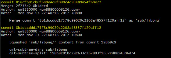
执行git status可以看到提示新增两条commit：

image

git log查看详细修改：

image

执行git push把修改推送到远端photoshop仓库，现在本地仓库与远端仓库的目录结构为：

photoshop
    |
    |-- sub/
    |   |
    |   \--libpng/
    |       |
    |       |-- libpng.c
    |       |-- libpng.h
    |       \-- README.md
    |
    |-- photoshop.c
    |-- photoshop.h
    |-- main.c
    \-- README.md

注意，现在的photoshop仓库对于其他项目人员来说，可以不需要知道libpng是一个子仓库。什么意思呢？
当你git clone或者git pull的时候，你拉取到的是整个photoshop(包括libpng在内，libpng就相当于photoshop里的一个普通目录)；当你修改了libpng里的内容后执行git push，你将会把修改push到photoshop上。
也就是说photoshop仓库下的libpng与其他文件无异。

从源仓库拉取更新

如果源libpng仓库更新了，photoshop里的libpng如何拉取更新？使用git subtree pull，例如：

1	git subtree pull --prefix=sub/libpng https://github.com/test/libpng.git master --squash

推送修改到源仓库

如果在photoshop仓库里修改了libpng，然后想把这个修改推送到源libpng仓库呢？使用git subtree push，例如：

1	git subtree push --prefix=sub/libpng https://github.com/test/libpng.git master

简化git subtree命令

我们已经知道了git subtree 的命令的基本用法，但是上述几个命令还是显得有点复杂，特别是子仓库的源仓库地址，特别不方便记忆。
这里我们把子仓库的地址作为一个remote，方便记忆：

1	git remote add -f libpng https://github.com/test/libpng.git

然后可以这样来使用git subtree命令：

1
2
3

git subtree add --prefix=sub/libpng libpng master --squash
git subtree pull --prefix=sub/libpng libpng master --squash
git subtree push --prefix=sub/libpng libpng master

Wed Jul 24 2019 00:00:00 GMT+0800 (China Standard Time)

发表于 2019-07-24 更新于 2026-03-05

时序数据库InfluxDB使用详解

发表于 2019-07-20 更新于 2026-03-05 分类于数据库， InfluxDB

InfluxDB是一个开源的时序数据库，使用GO语言开发，特别适合用于处理和分析资源监控数据这种时序相关数据。而InfluxDB自带的各种特殊函数如求标准差，随机取样数据，统计数据变化比等，使数据统计和实时分析变得十分方便。在我们的容器资源监控系统中，就采用了InfluxDB存储cadvisor的监控数据。本文对InfluxDB的基本概念和一些特色功能做一个详细介绍，内容主要是翻译整理自官网文档，如有错漏，请指正。

这里说一下使用docker容器运行influxdb的步骤，物理机安装请参照官方文档。拉取镜像文件后运行即可，当前最新版本是1.3.5。启动容器时设置挂载的数据目录和开放端口。InfluxDB的操作语法InfluxQL与SQL基本一致，也提供了一个类似mysql-client的名为influx的CLI。InfluxDB本身是支持分布式部署多副本存储的，本文介绍都是针对的单节点单副本。



f216e9be15bff545befecb30d1d275552026216a939cc20c042b17419e3bde31

root@f216e9be15bf:/
Connected to http:
InfluxDB shell version: 1.3.5
> create database cadvisor  
> show databases           
name: databases
name
----
_internal
cadvisor
> CREATE USER testuser WITH PASSWORD 'testpwd' 
> GRANT ALL PRIVILEGES ON cadvisor TO testuser 
> CREATE RETENTION POLICY "cadvisor_retention" ON "cadvisor" DURATION 30d REPLICATION 1 DEFAULT

influxdb里面有一些重要概念：database，timestamp，field key， field value， field set，tag key，tag value，tag set，measurement， retention policy ，series，point。结合下面的例子数据来说明这几个概念：

name: census
-————————————
time                     butterflies     honeybees     location   scientist
2015-08-18T00:00:00Z      12                23           1         langstroth
2015-08-18T00:00:00Z      1                 30           1         perpetua
2015-08-18T00:06:00Z      11                28           1         langstroth
2015-08-18T00:06:00Z      3                 28           1         perpetua
2015-08-18T05:54:00Z      2                 11           2         langstroth
2015-08-18T06:00:00Z      1                 10           2         langstroth
2015-08-18T06:06:00Z      8                 23           2         perpetua
2015-08-18T06:12:00Z      7                 22           2         perpetua

timestamp

既然是时间序列数据库，influxdb的数据都有一列名为time的列，里面存储UTC时间戳。

field key，field value，field set

butterflies和honeybees两列数据称为字段(fields)，influxdb的字段由field key和field value组成。其中butterflies和honeybees为field key，它们为string类型，用于存储元数据。

而butterflies这一列的数据12-7为butterflies的field value，同理，honeybees这一列的23-22为honeybees的field value。field value可以为string，float，integer或boolean类型。field value通常都是与时间关联的。

field key和field value对组成的集合称之为field set。如下：

butterflies = 12 honeybees = 23
butterflies = 1 honeybees = 30
butterflies = 11 honeybees = 28
butterflies = 3 honeybees = 28
butterflies = 2 honeybees = 11
butterflies = 1 honeybees = 10
butterflies = 8 honeybees = 23
butterflies = 7 honeybees = 22

在influxdb中，字段必须存在。注意，字段是没有索引的。如果使用字段作为查询条件，会扫描符合查询条件的所有字段值，性能不及tag。类比一下，fields相当于SQL的没有索引的列。

tag key，tag value，tag set

location和scientist这两列称为标签(tags)，标签由tag key和tag value组成。location这个tag key有两个tag value：1和2，scientist有两个tag value：langstroth和perpetua。tag key和tag value对组成了tag set，示例中的tag set如下：

location = 1, scientist = langstroth
location = 2, scientist = langstroth
location = 1, scientist = perpetua
location = 2, scientist = perpetua

tags是可选的，但是强烈建议你用上它，因为tag是有索引的，tags相当于SQL中的有索引的列。tag value只能是string类型 如果你的常用场景是根据butterflies和honeybees来查询，那么你可以将这两个列设置为tag，而其他两列设置为field，tag和field依据具体查询需求来定。

measurement

measurement是fields，tags以及time列的容器，measurement的名字用于描述存储在其中的字段数据，类似mysql的表名。如上面例子中的measurement为census。measurement相当于SQL中的表，本文中我在部分地方会用表来指代measurement。

retention policy

retention policy指数据保留策略，示例数据中的retention policy为默认的autogen。它表示数据一直保留永不过期，副本数量为1。你也可以指定数据的保留时间，如30天。

series

series是共享同一个retention policy，measurement以及tag set的数据集合。示例中数据有4个series，如下:

Arbitrary series number

Retention policy

Measurement

Tag set

series 1

autogen

census

location = 1,scientist = langstroth

series 2

autogen

census

location = 2,scientist = langstroth

series 3

autogen

census

location = 1,scientist = perpetua

series 4

autogen

census

location = 2,scientist = perpetua

point

point则是同一个series中具有相同时间的field set，points相当于SQL中的数据行。如下面就是一个point：

name: census
-----------------
time                  butterflies    honeybees   location    scientist
2015-08-18T00:00:00Z       1            30           1        perpetua

database

上面提到的结构都存储在数据库中，示例的数据库为my_database。一个数据库可以有多个measurement，retention policy， continuous queries以及user。influxdb是一个无模式的数据库，可以很容易的添加新的measurement，tags，fields等。而它的操作却和传统的数据库一样，可以使用类SQL语言查询和修改数据。

influxdb不是一个完整的CRUD数据库，它更像是一个CR-ud数据库。它优先考虑的是增加和读取数据而不是更新和删除数据的性能，而且它阻止了某些更新和删除行为使得创建和读取数据更加高效。

influxdb函数分为聚合函数，选择函数，转换函数，预测函数等。除了与普通数据库一样提供了基本操作函数外，还提供了一些特色函数以方便数据统计计算，下面会一一介绍其中一些常用的特色函数。

聚合函数：FILL(), INTEGRAL()，SPREAD()， STDDEV()，MEAN(), MEDIAN()等。
选择函数: SAMPLE(), PERCENTILE(), FIRST(), LAST(), TOP(), BOTTOM()等。
转换函数: DERIVATIVE(), DIFFERENCE()等。
预测函数：HOLT_WINTERS()。

先从官网导入测试数据（注：这里测试用的版本是1.3.1，最新版本是1.3.5）:

$ curl https://s3.amazonaws.com/noaa.water-database/NOAA_data.txt -o NOAA_data.txt
$ influx -import -path=NOAA_data.txt -precision=s -database=NOAA_water_database
$ influx -precision rfc3339 -database NOAA_water_database
Connected to http://localhost:8086 version 1.3.1
InfluxDB shell 1.3.1
> show measurements
name: measurements
name
----
average_temperature
distincts
h2o_feet
h2o_pH
h2o_quality
h2o_temperature

> show series from h2o_feet;
key
---
h2o_feet,location=coyote_creek
h2o_feet,location=santa_monica

下面的例子都以官方示例数据库来测试，这里只用部分数据以方便观察。measurement为h2o_feet，tag key为location，field key有level description和water_level两个。

> SELECT * FROM "h2o_feet" WHERE time >= '2015-08-17T23:48:00Z' AND time <= '2015-08-18T00:30:00Z'
name: h2o_feet
time                 level description    location     water_level
----                 -----------------    --------     -----------
2015-08-18T00:00:00Z between 6 and 9 feet coyote_creek 8.12
2015-08-18T00:00:00Z below 3 feet         santa_monica 2.064
2015-08-18T00:06:00Z between 6 and 9 feet coyote_creek 8.005
2015-08-18T00:06:00Z below 3 feet         santa_monica 2.116
2015-08-18T00:12:00Z between 6 and 9 feet coyote_creek 7.887
2015-08-18T00:12:00Z below 3 feet         santa_monica 2.028
2015-08-18T00:18:00Z between 6 and 9 feet coyote_creek 7.762
2015-08-18T00:18:00Z below 3 feet         santa_monica 2.126
2015-08-18T00:24:00Z between 6 and 9 feet coyote_creek 7.635
2015-08-18T00:24:00Z below 3 feet         santa_monica 2.041
2015-08-18T00:30:00Z between 6 and 9 feet coyote_creek 7.5
2015-08-18T00:30:00Z below 3 feet         santa_monica 2.051

GROUP BY，FILL()

如下语句中GROUP BY time(12m),* 表示以每12分钟和tag(location)分组(如果是GROUP BY time(12m)则表示仅每12分钟分组，GROUP BY 参数只能是time和tag)。然后fill(200)表示如果这个时间段没有数据，以200填充，mean(field_key)求该范围内数据的平均值(注意：这是依据series来计算。其他还有SUM求和，MEDIAN求中位数)。LIMIT 7表示限制返回的point(记录数)最多为7条，而SLIMIT 1则是限制返回的series为1个。

注意这里的时间区间，起始时间为整点前包含这个区间第一个12m的时间，比如这里为 2015-08-17T:23:48:00Z，第一条为 2015-08-17T23:48:00Z <= t < 2015-08-18T00:00:00Z这个区间的location=coyote_creek的water_level的平均值，这里没有数据，于是填充的200。第二条为 2015-08-18T00:00:00Z <= t < 2015-08-18T00:12:00Z区间的location=coyote_creek的water_level平均值，这里为 （8.12+8.005）/ 2 = 8.0625，其他以此类推。

而GROUP BY time(10m)则表示以10分钟分组，起始时间为包含这个区间的第一个10m的时间，即 2015-08-17T23:40:00Z。默认返回的是第一个series，如果要计算另外那个series，可以在SQL语句后面加上 SOFFSET 1。

那如果时间小于数据本身采集的时间间隔呢，比如GROUP BY time(10s)呢？这样的话，就会按10s取一个点，没有数值的为空或者FILL填充，对应时间点有数据则保持不变。

## GROUP BY time(12m)
> SELECT mean("water_level") FROM "h2o_feet" WHERE time >= '2015-08-17T23:48:00Z' AND time <= '2015-08-18T00:30:00Z' GROUP BY time(12m),* fill(200) LIMIT 7 SLIMIT 1
name: h2o_feet
tags: location=coyote_creek
time                 mean
----                 ----
2015-08-17T23:48:00Z 200
2015-08-18T00:00:00Z 8.0625
2015-08-18T00:12:00Z 7.8245
2015-08-18T00:24:00Z 7.5675

## GROUP BY time(10m)，SOFFSET设置为1
> SELECT mean("water_level") FROM "h2o_feet" WHERE time >= '2015-08-17T23:48:00Z' AND time <= '2015-08-18T00:30:00Z' GROUP BY time(10m),* fill(200) LIMIT 7 SLIMIT 1 SOFFSET 1
name: h2o_feet
tags: location=santa_monica
time                 mean
----                 ----
2015-08-17T23:40:00Z 200
2015-08-17T23:50:00Z 200
2015-08-18T00:00:00Z 2.09
2015-08-18T00:10:00Z 2.077
2015-08-18T00:20:00Z 2.041
2015-08-18T00:30:00Z 2.051

INTEGRAL(field_key, unit)

计算数值字段值覆盖的曲面的面积值并得到面积之和。测试数据如下：

> SELECT "water_level" FROM "h2o_feet" WHERE "location" = 'santa_monica' AND time >= '2015-08-18T00:00:00Z' AND time <= '2015-08-18T00:30:00Z'

name: h2o_feet
time                   water_level
----                   -----------
2015-08-18T00:00:00Z   2.064
2015-08-18T00:06:00Z   2.116
2015-08-18T00:12:00Z   2.028
2015-08-18T00:18:00Z   2.126
2015-08-18T00:24:00Z   2.041
2015-08-18T00:30:00Z   2.051

使用INTERGRAL计算面积。注意，这个面积就是这些点连接起来后与时间围成的不规则图形的面积，注意unit默认是以1秒计算，所以下面语句计算结果为3732.66=2.028*1800+分割出来的梯形和三角形面积。如果unit改为1分，则结果为3732.66/60 = 62.211。unit为2分，则结果为3732.66/120 = 31.1055。以此类推。

# unit为默认的1秒
> SELECT INTEGRAL("water_level") FROM "h2o_feet" WHERE "location" = 'santa_monica' AND time >= '2015-08-18T00:00:00Z' AND time <= '2015-08-18T00:30:00Z'
name: h2o_feet
time                 integral
----                 --------
1970-01-01T00:00:00Z 3732.66

# unit为1分
> SELECT INTEGRAL("water_level", 1m) FROM "h2o_feet" WHERE "location" = 'santa_monica' AND time >= '2015-08-18T00:00:00Z' AND time <= '2015-08-18T00:30:00Z'
name: h2o_feet
time                 integral
----                 --------
1970-01-01T00:00:00Z 62.211

SPREAD(field_key)

计算数值字段的最大值和最小值的差值。

> SELECT SPREAD("water_level") FROM "h2o_feet" WHERE time >= '2015-08-17T23:48:00Z' AND time <= '2015-08-18T00:30:00Z' GROUP BY time(12m),* fill(18) LIMIT 3 SLIMIT 1 SOFFSET 1
name: h2o_feet
tags: location=santa_monica
time                 spread
----                 ------
2015-08-17T23:48:00Z 18
2015-08-18T00:00:00Z 0.052000000000000046
2015-08-18T00:12:00Z 0.09799999999999986

STDDEV(field_key)

计算字段的标准差。influxdb用的是贝塞尔修正的标准差计算公式，如下：

mean=(v1+v2+…+vn)/n;
stddev = math.sqrt(
((v1-mean)2 + (v2-mean)2 + …+(vn-mean)2)/(n-1)
)

> SELECT STDDEV("water_level") FROM "h2o_feet" WHERE time >= '2015-08-17T23:48:00Z' AND time <= '2015-08-18T00:30:00Z' GROUP BY time(12m),* fill(18) SLIMIT 1;
name: h2o_feet
tags: location=coyote_creek
time                 stddev
----                 ------
2015-08-17T23:48:00Z 18
2015-08-18T00:00:00Z 0.08131727983645186
2015-08-18T00:12:00Z 0.08838834764831845
2015-08-18T00:24:00Z 0.09545941546018377

PERCENTILE(field_key, N)

选取某个字段中大于N%的这个字段值。

如果一共有4条记录，N为10，则10%*4=0.4，四舍五入为0，则查询结果为空。N为20，则 20% * 4 = 0.8，四舍五入为1，选取的是4个数中最小的数。如果N为40，40% * 4 = 1.6，四舍五入为2，则选取的是4个数中第二小的数。由此可以看出N=100时，就跟MAX(field_key)是一样的，而当N=50时，与MEDIAN(field_key)在字段值为奇数个时是一样的。

> SELECT PERCENTILE("water_level",20) FROM "h2o_feet" WHERE time >= '2015-08-17T23:48:00Z' AND time <= '2015-08-18T00:30:00Z' GROUP BY time(12m)
name: h2o_feet
time                 percentile
----                 ----------
2015-08-17T23:48:00Z 
2015-08-18T00:00:00Z 2.064
2015-08-18T00:12:00Z 2.028
2015-08-18T00:24:00Z 2.041

> SELECT PERCENTILE("water_level",40) FROM "h2o_feet" WHERE time >= '2015-08-17T23:48:00Z' AND time <= '2015-08-18T00:30:00Z' GROUP BY time(12m)
name: h2o_feet
time                 percentile
----                 ----------
2015-08-17T23:48:00Z 
2015-08-18T00:00:00Z 2.116
2015-08-18T00:12:00Z 2.126
2015-08-18T00:24:00Z 2.051

SAMPLE(field_key, N)

随机返回field key的N个值。如果语句中有GROUP BY time()，则每组数据随机返回N个值。

> SELECT SAMPLE("water_level",2) FROM "h2o_feet" WHERE time >= '2015-08-17T23:48:00Z' AND time <= '2015-08-18T00:30:00Z';
name: h2o_feet
time                 sample
----                 ------
2015-08-18T00:00:00Z 2.064
2015-08-18T00:12:00Z 2.028

> SELECT SAMPLE("water_level",2) FROM "h2o_feet" WHERE time >= '2015-08-17T23:48:00Z' AND time <= '2015-08-18T00:30:00Z' GROUP BY time(12m);
name: h2o_feet
time                 sample
----                 ------
2015-08-18T00:06:00Z 2.116
2015-08-18T00:06:00Z 8.005
2015-08-18T00:12:00Z 7.887
2015-08-18T00:18:00Z 7.762
2015-08-18T00:24:00Z 7.635
2015-08-18T00:30:00Z 2.051

CUMULATIVE_SUM(field_key)

计算字段值的递增和。

> SELECT CUMULATIVE_SUM("water_level") FROM "h2o_feet" WHERE time >= '2015-08-17T23:48:00Z' AND time <= '2015-08-18T00:30:00Z';
name: h2o_feet
time                 cumulative_sum
----                 --------------
2015-08-18T00:00:00Z 8.12
2015-08-18T00:00:00Z 10.184
2015-08-18T00:06:00Z 18.189
2015-08-18T00:06:00Z 20.305
2015-08-18T00:12:00Z 28.192
2015-08-18T00:12:00Z 30.22
2015-08-18T00:18:00Z 37.982
2015-08-18T00:18:00Z 40.108
2015-08-18T00:24:00Z 47.742999999999995
2015-08-18T00:24:00Z 49.78399999999999
2015-08-18T00:30:00Z 57.28399999999999
2015-08-18T00:30:00Z 59.334999999999994

DERIVATIVE(field_key, unit) 和 NON_NEGATIVE_DERIVATIVE(field_key, unit)

计算字段值的变化比。unit默认为1s，即计算的是1秒内的变化比。

如下面的第一个数据计算方法是 (2.116-2.064)/(6*60) = 0.00014..，其他计算方式同理。虽然原始数据是6m收集一次，但是这里的变化比默认是按秒来计算的。如果要按6m计算，则设置unit为6m即可。

> SELECT DERIVATIVE("water_level") FROM "h2o_feet" WHERE "location" = 'santa_monica' AND time >= '2015-08-18T00:00:00Z' AND time <= '2015-08-18T00:30:00Z'
name: h2o_feet
time                 derivative
----                 ----------
2015-08-18T00:06:00Z 0.00014444444444444457
2015-08-18T00:12:00Z -0.00024444444444444465
2015-08-18T00:18:00Z 0.0002722222222222218
2015-08-18T00:24:00Z -0.000236111111111111
2015-08-18T00:30:00Z 0.00002777777777777842

> SELECT DERIVATIVE("water_level", 6m) FROM "h2o_feet" WHERE "location" = 'santa_monica' AND time >= '2015-08-18T00:00:00Z' AND time <= '2015-08-18T00:30:00Z'
name: h2o_feet
time                 derivative
----                 ----------
2015-08-18T00:06:00Z 0.052000000000000046
2015-08-18T00:12:00Z -0.08800000000000008
2015-08-18T00:18:00Z 0.09799999999999986
2015-08-18T00:24:00Z -0.08499999999999996
2015-08-18T00:30:00Z 0.010000000000000231

而DERIVATIVE结合GROUP BY time，以及mean可以构造更加复杂的查询，如下所示:

> SELECT DERIVATIVE(mean("water_level"), 6m) FROM "h2o_feet" WHERE time >= '2015-08-18T00:00:00Z' AND time <= '2015-08-18T00:30:00Z' group by time(12m), *
name: h2o_feet
tags: location=coyote_creek
time                 derivative
----                 ----------
2015-08-18T00:12:00Z -0.11900000000000022
2015-08-18T00:24:00Z -0.12849999999999984

name: h2o_feet
tags: location=santa_monica
time                 derivative
----                 ----------
2015-08-18T00:12:00Z -0.00649999999999995
2015-08-18T00:24:00Z -0.015499999999999847

这个计算其实是先根据GROUP BY time求平均值，然后对这个平均值再做变化比的计算。因为数据是按12分钟分组的，而变化比的unit是6分钟，所以差值除以2(12/6)才得到变化比。如第一个值是 (7.8245-8.0625)/2 = -0.1190。

> SELECT mean("water_level") FROM "h2o_feet" WHERE time >= '2015-08-18T00:00:00Z' AND time <= '2015-08-18T00:30:00Z' group by time(12m), *
name: h2o_feet
tags: location=coyote_creek
time                 mean
----                 ----
2015-08-18T00:00:00Z 8.0625
2015-08-18T00:12:00Z 7.8245
2015-08-18T00:24:00Z 7.5675

name: h2o_feet
tags: location=santa_monica
time                 mean
----                 ----
2015-08-18T00:00:00Z 2.09
2015-08-18T00:12:00Z 2.077
2015-08-18T00:24:00Z 2.0460000000000003

NON_NEGATIVE_DERIVATIVE与DERIVATIVE不同的是它只返回的是非负的变化比:

> SELECT DERIVATIVE(mean("water_level"), 6m) FROM "h2o_feet" WHERE location='santa_monica' AND time >= '2015-08-18T00:00:00Z' AND time <= '2015-08-18T00:30:00Z' group by time(6m), *
name: h2o_feet
tags: location=santa_monica
time                 derivative
----                 ----------
2015-08-18T00:06:00Z 0.052000000000000046
2015-08-18T00:12:00Z -0.08800000000000008
2015-08-18T00:18:00Z 0.09799999999999986
2015-08-18T00:24:00Z -0.08499999999999996
2015-08-18T00:30:00Z 0.010000000000000231

> SELECT NON_NEGATIVE_DERIVATIVE(mean("water_level"), 6m) FROM "h2o_feet" WHERE location='santa_monica' AND time >= '2015-08-18T00:00:00Z' AND time <= '2015-08-18T00:30:00Z' group by time(6m), *
name: h2o_feet
tags: location=santa_monica
time                 non_negative_derivative
----                 -----------------------
2015-08-18T00:06:00Z 0.052000000000000046
2015-08-18T00:18:00Z 0.09799999999999986
2015-08-18T00:30:00Z 0.010000000000000231

4.1 基本语法

连续查询(CONTINUOUS QUERY，简写为CQ)是指定时自动在实时数据上进行的InfluxQL查询，查询结果可以存储到指定的measurement中。基本语法格式如下：

CREATE CONTINUOUS QUERY <cq_name> ON <database_name>
BEGIN
  <cq_query>
END

cq_query格式：
SELECT <function[s]> INTO <destination_measurement> FROM <measurement> [WHERE <stuff>] GROUP BY time(<interval>)[,<tag_key[s]>]

CQ操作的是实时数据，它使用本地服务器的时间戳、GROUP BY time()时间间隔以及InfluxDB预先设置好的时间范围来确定什么时候开始查询以及查询覆盖的时间范围。注意CQ语句里面的WHERE条件是没有时间范围的，因为CQ会根据GROUP BY time()自动确定时间范围。

CQ执行的时间间隔和GROUP BY time()的时间间隔一样，它在InfluxDB预先设置的时间范围的起始时刻执行。如果GROUP BY time(1h)，则单次查询的时间范围为 now()-GROUP BY time(1h)到 now()，也就是说，如果当前时间为17点，这次查询的时间范围为 16:00到16:59.99999。

下面看几个示例，示例数据如下，这是数据库transportation中名为bus_data的measurement，每15分钟统计一次乘客数和投诉数。数据文件bus_data.txt如下：

# DDL
CREATE DATABASE transportation

# DML
# CONTEXT-DATABASE: transportation 

bus_data,complaints=9 passengers=5 1472367600
bus_data,complaints=9 passengers=8 1472368500
bus_data,complaints=9 passengers=8 1472369400
bus_data,complaints=9 passengers=7 1472370300
bus_data,complaints=9 passengers=8 1472371200
bus_data,complaints=7 passengers=15 1472372100
bus_data,complaints=7 passengers=15 1472373000
bus_data,complaints=7 passengers=17 1472373900
bus_data,complaints=7 passengers=20 1472374800

导入数据，命令如下：

root@f216e9be15bf:/# influx -import -path=bus_data.txt -precision=s
root@f216e9be15bf:/# influx -precision=rfc3339 -database=transportation
Connected to http://localhost:8086 version 1.3.5
InfluxDB shell version: 1.3.5
> select * from bus_data
name: bus_data
time                 complaints passengers
----                 ---------- ----------
2016-08-28T07:00:00Z 9          5
2016-08-28T07:15:00Z 9          8
2016-08-28T07:30:00Z 9          8
2016-08-28T07:45:00Z 9          7
2016-08-28T08:00:00Z 9          8
2016-08-28T08:15:00Z 7          15
2016-08-28T08:30:00Z 7          15
2016-08-28T08:45:00Z 7          17
2016-08-28T09:00:00Z 7          20

示例1 自动缩小取样存储到新的measurement中

对单个字段自动缩小取样并存储到新的measurement中。

CREATE CONTINUOUS QUERY "cq_basic" ON "transportation"
BEGIN
  SELECT mean("passengers") INTO "average_passengers" FROM "bus_data" GROUP BY time(1h)
END

这个CQ的意思就是对bus_data每小时自动计算取样数据的平均乘客数并存储到 average_passengers中。那么在2016-08-28这天早上会执行如下流程：

At 8:00 cq_basic 执行查询，查询时间范围 time >= '7:00' AND time < '08:00'.
cq_basic写入一条记录到 average_passengers:
name: average_passengers
------------------------
time                   mean
2016-08-28T07:00:00Z   7
At 9:00 cq_basic 执行查询，查询时间范围 time >= '8:00' AND time < '9:00'.
cq_basic写入一条记录到 average_passengers:
name: average_passengers
------------------------
time                   mean
2016-08-28T08:00:00Z   13.75

# Results
> SELECT * FROM "average_passengers"
name: average_passengers
------------------------
time                   mean
2016-08-28T07:00:00Z   7
2016-08-28T08:00:00Z   13.75

示例2 自动缩小取样并存储到新的保留策略（Retention Policy）中

CREATE CONTINUOUS QUERY "cq_basic_rp" ON "transportation"
BEGIN
  SELECT mean("passengers") INTO "transportation"."three_weeks"."average_passengers" FROM "bus_data" GROUP BY time(1h)
END

与示例1类似，不同的是保留的策略不是autogen，而是改成了three_weeks(创建保留策略语法 CREATE RETENTION POLICY "three_weeks" ON "transportation" DURATION 3w REPLICATION 1)。

> SELECT * FROM "transportation"."three_weeks"."average_passengers"
name: average_passengers
------------------------
time                   mean
2016-08-28T07:00:00Z   7
2016-08-28T08:00:00Z   13.75

示例3 使用后向引用(backreferencing)自动缩小取样并存储到新的数据库中

CREATE CONTINUOUS QUERY "cq_basic_br" ON "transportation"
BEGIN
  SELECT mean(*) INTO "downsampled_transportation"."autogen".:MEASUREMENT FROM /.*/ GROUP BY time(30m),*
END

使用后向引用语法自动缩小取样并存储到新的数据库中。语法 :MEASUREMENT 用来指代后面的表，而 /.*/则是分别查询所有的表。这句CQ的含义就是每30分钟自动查询transportation的所有表(这里只有bus_data一个表)，并将30分钟内数字字段(passengers和complaints)求平均值存储到新的数据库 downsampled_transportation中。

最终结果如下：

> SELECT * FROM "downsampled_transportation."autogen"."bus_data"
name: bus_data
--------------
time                   mean_complaints   mean_passengers
2016-08-28T07:00:00Z   9                 6.5
2016-08-28T07:30:00Z   9                 7.5
2016-08-28T08:00:00Z   8                 11.5
2016-08-28T08:30:00Z   7                 16

示例4 自动缩小取样以及配置CQ的时间范围

CREATE CONTINUOUS QUERY "cq_basic_offset" ON "transportation"
BEGIN
  SELECT mean("passengers") INTO "average_passengers" FROM "bus_data" GROUP BY time(1h,15m)
END

与前面几个示例不同的是，这里的GROUP BY time(1h, 15m)指定了一个时间偏移，也就是说 cq_basic_offset执行的时间不再是整点，而是往后偏移15分钟。执行流程如下:

At 8:15 cq_basic_offset 执行查询的时间范围 time >= '7:15' AND time < '8:15'.
name: average_passengers
------------------------
time                   mean
2016-08-28T07:15:00Z   7.75
At 9:15 cq_basic_offset 执行查询的时间范围 time >= '8:15' AND time < '9:15'.
name: average_passengers
------------------------
time                   mean
2016-08-28T08:15:00Z   16.75

最终结果:

> SELECT * FROM "average_passengers"
name: average_passengers
------------------------
time                   mean
2016-08-28T07:15:00Z   7.75
2016-08-28T08:15:00Z   16.75

4.2 高级语法

InfluxDB连续查询的高级语法如下：

CREATE CONTINUOUS QUERY <cq_name> ON <database_name>
RESAMPLE EVERY <interval> FOR <interval>
BEGIN
  <cq_query>
END

与基本语法不同的是，多了RESAMPLE关键字。高级语法里CQ的执行时间和查询时间范围则与RESAMPLE里面的两个interval有关系。

高级语法中CQ以EVERY interval的时间间隔执行，执行时查询的时间范围则是FOR interval来确定。如果FOR interval为2h，当前时间为17:00，则查询的时间范围为15:00-16:59.999999。RESAMPLE的EVERY和FOR两个关键字可以只有一个。

示例的数据表如下，比之前的多了几条记录为了示例3和示例4的测试:

name: bus_data
--------------
time                   passengers
2016-08-28T06:30:00Z   2
2016-08-28T06:45:00Z   4
2016-08-28T07:00:00Z   5
2016-08-28T07:15:00Z   8
2016-08-28T07:30:00Z   8
2016-08-28T07:45:00Z   7
2016-08-28T08:00:00Z   8
2016-08-28T08:15:00Z   15
2016-08-28T08:30:00Z   15
2016-08-28T08:45:00Z   17
2016-08-28T09:00:00Z   20

示例1 只配置执行时间间隔

CREATE CONTINUOUS QUERY "cq_advanced_every" ON "transportation"
RESAMPLE EVERY 30m
BEGIN
  SELECT mean("passengers") INTO "average_passengers" FROM "bus_data" GROUP BY time(1h)
END

这里配置了30分钟执行一次CQ，没有指定FOR interval，于是查询的时间范围还是GROUP BY time(1h)指定的一个小时，执行流程如下：

At 8:00, cq_advanced_every 执行时间范围 time >= '7:00' AND time < '8:00'.
name: average_passengers
------------------------
time                   mean
2016-08-28T07:00:00Z   7
At 8:30, cq_advanced_every 执行时间范围 time >= '8:00' AND time < '9:00'.
name: average_passengers
------------------------
time                   mean
2016-08-28T08:00:00Z   12.6667
At 9:00, cq_advanced_every 执行时间范围 time >= '8:00' AND time < '9:00'.
name: average_passengers
------------------------
time                   mean
2016-08-28T08:00:00Z   13.75

需要注意的是，这里的 8点到9点这个区间执行了两次，第一次执行时时8:30，平均值是 (8+15+15）/ 3 = 12.6667，而第二次执行时间是9:00，平均值是 (8+15+15+17) / 4=13.75，而且最后第二个结果覆盖了第一个结果。InfluxDB如何处理重复的记录可以参见这个文档。

最终结果：

> SELECT * FROM "average_passengers"
name: average_passengers
------------------------
time                   mean
2016-08-28T07:00:00Z   7
2016-08-28T08:00:00Z   13.75

示例2 只配置查询时间范围

CREATE CONTINUOUS QUERY "cq_advanced_for" ON "transportation"
RESAMPLE FOR 1h
BEGIN
  SELECT mean("passengers") INTO "average_passengers" FROM "bus_data" GROUP BY time(30m)
END

只配置了时间范围，而没有配置EVERY interval。这样，执行的时间间隔与GROUP BY time(30m)一样为30分钟，而查询的时间范围为1小时，由于是按30分钟分组，所以每次会写入两条记录。执行流程如下：

At 8:00 cq_advanced_for 查询时间范围：time >= '7:00' AND time < '8:00'.
写入两条记录。
name: average_passengers
------------------------
time                   mean
2016-08-28T07:00:00Z   6.5
2016-08-28T07:30:00Z   7.5
At 8:30 cq_advanced_for 查询时间范围：time >= '7:30' AND time < '8:30'.
写入两条记录。
name: average_passengers
------------------------
time                   mean
2016-08-28T07:30:00Z   7.5
2016-08-28T08:00:00Z   11.5
At 9:00 cq_advanced_for 查询时间范围：time >= '8:00' AND time < '9:00'.
写入两条记录。
name: average_passengers
------------------------
time                   mean
2016-08-28T08:00:00Z   11.5
2016-08-28T08:30:00Z   16

需要注意的是，cq_advanced_for每次写入了两条记录，重复的记录会被覆盖。

最终结果：

> SELECT * FROM "average_passengers"
name: average_passengers
------------------------
time                   mean
2016-08-28T07:00:00Z   6.5
2016-08-28T07:30:00Z   7.5
2016-08-28T08:00:00Z   11.5
2016-08-28T08:30:00Z   16

示例3 同时配置执行时间间隔和查询时间范围

CREATE CONTINUOUS QUERY "cq_advanced_every_for" ON "transportation"
RESAMPLE EVERY 1h FOR 90m
BEGIN
  SELECT mean("passengers") INTO "average_passengers" FROM "bus_data" GROUP BY time(30m)
END

这里配置了执行间隔为1小时，而查询范围90分钟，最后分组是30分钟，每次插入了三条记录。执行流程如下：

At 8:00 cq_advanced_every_for 查询时间范围 time >= '6:30' AND time < '8:00'.
插入三条记录
name: average_passengers
------------------------
time                   mean
2016-08-28T06:30:00Z   3
2016-08-28T07:00:00Z   6.5
2016-08-28T07:30:00Z   7.5
At 9:00 cq_advanced_every_for 查询时间范围 time >= '7:30' AND time < '9:00'.
插入三条记录
name: average_passengers
------------------------
time                   mean
2016-08-28T07:30:00Z   7.5
2016-08-28T08:00:00Z   11.5
2016-08-28T08:30:00Z   16

最终结果：

> SELECT * FROM "average_passengers"
name: average_passengers
------------------------
time                   mean
2016-08-28T06:30:00Z   3
2016-08-28T07:00:00Z   6.5
2016-08-28T07:30:00Z   7.5
2016-08-28T08:00:00Z   11.5
2016-08-28T08:30:00Z   16

示例4 配置查询时间范围和FILL填充

CREATE CONTINUOUS QUERY "cq_advanced_for_fill" ON "transportation"
RESAMPLE FOR 2h
BEGIN
  SELECT mean("passengers") INTO "average_passengers" FROM "bus_data" GROUP BY time(1h) fill(1000)
END

在前面值配置查询时间范围的基础上，加上FILL填充空的记录。执行流程如下：

At 6:00, cq_advanced_for_fill 查询时间范围：time >= '4:00' AND time < '6:00'，没有数据，不填充。

At 7:00, cq_advanced_for_fill 查询时间范围：time >= '5:00' AND time < '7:00'. 写入两条记录，没有数据的时间点填充1000。
------------------------
time                   mean
2016-08-28T05:00:00Z   1000          <------ fill(1000)
2016-08-28T06:00:00Z   3             <------ average of 2 and 4

[…] At 11:00, cq_advanced_for_fill 查询时间范围：time >= '9:00' AND time < '11:00'.写入两条记录，没有数据的点填充1000。
name: average_passengers
------------------------
2016-08-28T09:00:00Z   20            <------ average of 20
2016-08-28T10:00:00Z   1000          <------ fill(1000)     

At 12:00, cq_advanced_for_fill 查询时间范围：time >= '10:00' AND time < '12:00'。没有数据，不填充。

最终结果:

> SELECT * FROM "average_passengers"
name: average_passengers
------------------------
time                   mean
2016-08-28T05:00:00Z   1000
2016-08-28T06:00:00Z   3
2016-08-28T07:00:00Z   7
2016-08-28T08:00:00Z   13.75
2016-08-28T09:00:00Z   20
2016-08-28T10:00:00Z   1000

Fri Jul 19 2019 00:00:00 GMT+0800 (China Standard Time)

发表于 2019-07-19 更新于 2026-03-05

Sun Jul 14 2019 00:00:00 GMT+0800 (China Standard Time)

发表于 2019-07-14 更新于 2026-03-05

启动wpa_supplicant应用

启动wpa_cli应用

分配ip/netmask/gateway/dns

保存连接

断开连接

连接已有的连接

断开wifi

wpa_wifi_tool使用方法

准备

在父仓库中新增子仓库

从源仓库拉取更新

推送修改到源仓库

简化git subtree命令

timestamp

field key，field value，field set

tag key，tag value，tag set

measurement

retention policy

series

point

database

GROUP BY，FILL()

INTEGRAL(field_key, unit)

SPREAD(field_key)

STDDEV(field_key)

PERCENTILE(field_key, N)

SAMPLE(field_key, N)

CUMULATIVE_SUM(field_key)

DERIVATIVE(field_key, unit) 和 NON_NEGATIVE_DERIVATIVE(field_key, unit)

4.1 基本语法

示例1 自动缩小取样存储到新的measurement中

示例2 自动缩小取样并存储到新的保留策略（Retention Policy）中

示例3 使用后向引用(backreferencing)自动缩小取样并存储到新的数据库中

示例4 自动缩小取样以及配置CQ的时间范围

4.2 高级语法

示例1 只配置执行时间间隔

示例2 只配置查询时间范围

示例3 同时配置执行时间间隔和查询时间范围

示例4 配置查询时间范围和FILL填充

启动`wpa_supplicant`应用

启动`wpa_cli`应用

分配`ip/netmask/gateway/dns`

断开`wifi`

`wpa_wifi_tool`使用方法